1. File Menu

1. New

Creates a new view window on screen. The New View dialog appears:

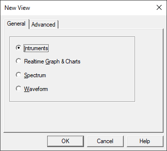
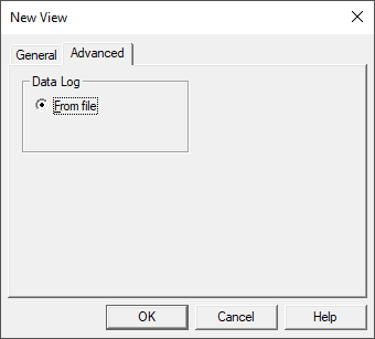
Figure 17 — Creating a new window (General and Advanced tabs)

On the General tab, choose the type of window to create: Instruments, Graph, Harmonic Spectrum or Harmonic Waveform. The Advanced tab is used to create a Data Log From File window.

Select the item you want and press .

1. Choosing Instrument

Creates a window that shows the values from the meters as numbers. The details are as follows.

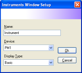
Figure 18 — Components of the Instrument window setup

The dialog contains:

1. Name — the name of the window, entered as text.

2. Device — the data source, as configured under File → Device Setup.

Display Type sets the kind of data to be shown. What appears here varies with the device connected.

2. Choosing Graph

Creates a trend graph view window, in which the conditions and the type of data required can be configured, as shown.

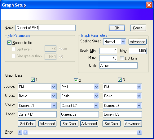
Figure 19 — Components of the trend graph window setup

The dialog has two parts.

General settings

1. Name — the name of the window, entered as text.

2. Record to file — whether the graph being created should store its data so that it can be reviewed later. It is normally ticked, so that historical graph values can be viewed.

3. Split every — splits the recorded graph data into separate parts after the given number of hours (no longer used).

4. Size greater than — as item 3, but splits the graph data when the stored file exceeds the given size (no longer used).

5. Scaling Style — how the Y axis presents the data. Normal is the usual case, where you set the min and max yourself; PF handles power factor as a special case; Digital displays digital inputs.

6. Advanced — see below.

7. Scale Min — the value at the bottom of the Y axis.

8. Scale Max — the value at the top of the Y axis.

9. Scale Major — the minor divisions along the Y axis. Enter 0 to have the program work them out automatically.

10. Dot Line — draws the graph grid as dots rather than solid lines.

11. Units — the unit text that appears against the Y axis.

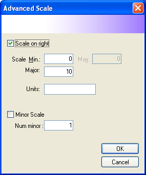
Figure 20 — Advanced Scale

The following appear when the Advanced button in Graph Parameters is pressed.

1. Scale on right — whether to show a second axis on the right-hand side. Normally the program shows only the left-hand axis. Each line must also be set to reference either the left or the right axis.

2. Scale Min, Max — the range of the right-hand Y axis.

3. Major — the step between Y axis divisions.

4. Units — the unit of the data.

5. Minor Scale — whether the program should draw lines between the main Y axis divisions.

6. Num minor — how many such lines to draw.

Settings for each graph line (Graph Data)

1. The numbered buttons with tick boxes turn the display of that line on and off.

2. Source — the data source as configured under File → Device Setup, or a calculated value; see "Calculations in a graph".

3. Group — the data group, which divides the values available in the system into manageable sets.

4. Value — the electrical value to plot as the graph line. Which values are offered depends on the source chosen in item 19.

5. Label — the text to show on the graph. You can edit it to whatever is most meaningful; by default it matches Value.

6. Set Color — sets the colour of the graph line yourself. The dialog below appears; choose the colour you want and press .

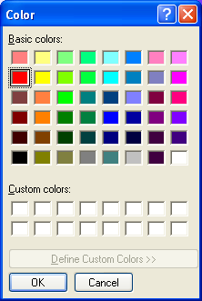
Figure 21 — Graph colour selection dialog

1. Advanced — further settings for each graph line, as follows.

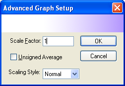
Figure 22 — Advanced Graph Setup

1. Scale Factor — a multiplier that determines where this line sits relative to the maximum scale. It is normally 1. For example, power factor runs between -1 and 1, so a factor is needed to display it usefully when the maximum scale is 100. It works equally well for other values, to make the graph easier to read and better looking.

2. Unsigned Average — tells the system to use absolute values only when averaging this line. This works particularly well for power factor.

3. Scaling Style — whether the line references the left or the right Y axis, in the case where the graph has been set to show two axes.

4. Page — selects which set of graph lines to configure; there are up to 16 sets of line definitions in total.

Once the basic graph settings are complete, press and the graph window appears on screen.

Notes

1. The graph window just created has not been saved. To save it, use File → Save or .

2. To change the graph settings later, use View → View Setup or .

Calculations in a graph

Selecting Formula as the source makes real-time calculated formulas available.

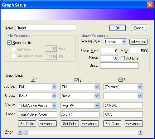
Figure 23 — Example of a formula used in a graph

The illustration shows a formula calculating KVA. Other examples:

5.3+(@1*60) — if channel 1 is set to voltage, it can be multiplied by the CT ratio (60) to give the high voltage, then offset by a constant (5.3) to give the high voltage as it should read.

Graphing system flags, or PLC / I/O module inputs and outputs

Variables that hold an on or off state are represented in the program as 1 = On, -1 = Off and 0 = Unstable. Graphs and setpoints built on them should be configured to match.

3. Choosing Harmonic Spectrum

Creates a window showing the harmonic spectrum from the meter, breaking out the percentage of each harmonic order, for those meter models that can measure it. The details are as follows.

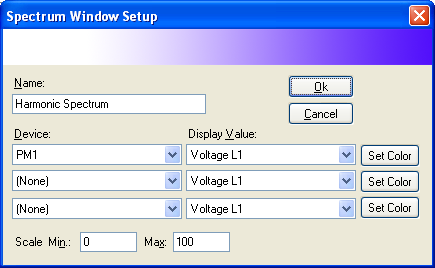
Figure 24 — Settings for creating a Harmonic Spectrum window

The dialog contains:

1. Name — the name of the window, entered as text.

2. Device — the data source, as configured under File → Device Setup, limited to devices capable of harmonics. Several values can be shown at once, from a single powermeter or from different ones.

3. Display Value — which electrical value the window shows the harmonic spectrum for; see the table below.

4. Scale Min and Scale Max — the range of the graph's Y axis.

5. Set Color — gives each displayed value a distinct colour.

Table 4 — Meaning of each display type

Display Type	Meaning
Voltage L1	Harmonic spectrum of voltage line 1, or 12
Voltage L2	Harmonic spectrum of voltage line 2, or 23
Voltage L3	Harmonic spectrum of voltage line 3, or 31
Current L1	Harmonic spectrum of current line 1, or 12
Current L2	Harmonic spectrum of current line 2, or 23
Current L3	Harmonic spectrum of current line 3, or 31

4. Choosing Harmonic Waveform

Creates a window showing the harmonic waveform from the meter, presented as the standard waveform with the harmonic distortion already combined into it. The details are as follows.

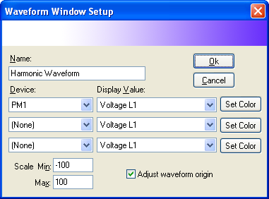
Figure 25 — Settings for creating a Harmonic Waveform window

The dialog contains:

1. Name — the name of the window, entered as text.

2. Device — the data source, as configured under File → Device Setup, limited to devices capable of harmonics. Several values can be shown at once, from a single powermeter or from different ones.

3. Display Value — which electrical value the window shows the harmonic waveform for; the options are the same as in the Harmonic Spectrum table above.

4. Adjust Waveform origin — whether the program should start the waveform at the positive half cycle, or draw it exactly as received.

5. Scale Min and Scale Max — the range of the graph's Y axis.

6. Set Color — gives each displayed value a distinct colour.

5. Choosing Data Log From File (on the Advanced tab)

Creates a window showing data that was held in the memory of a Digital Powermeter and has since been uploaded into a file. Select the Advanced tab in the New View dialog. The details are as follows.

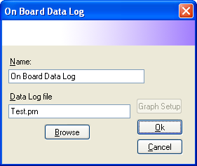
Figure 26 — On Board Data Log window setup

The dialog contains:

1. Name — the name of the window, entered as text.

2. Data Log file — the name of the file to display; use Browse to select it.

3. Graph Setup — a button that opens the graph display settings (see Figure 28, On Board Graph Setup).

The result is displayed as shown.

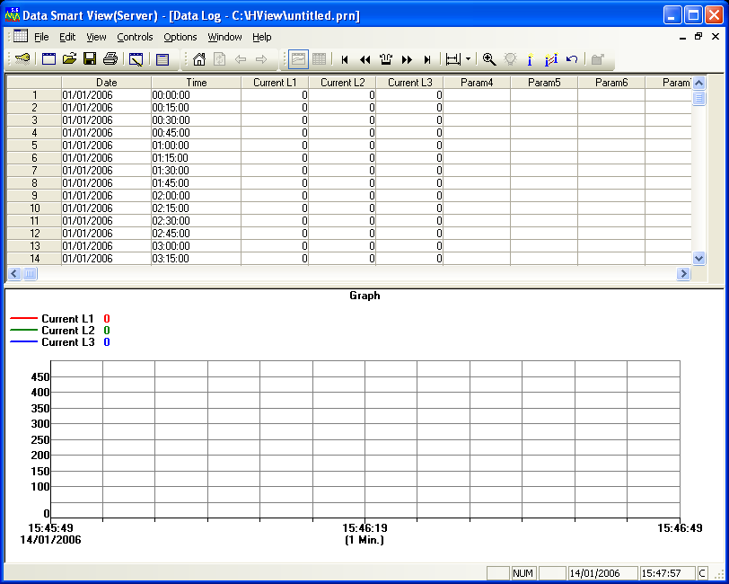
Figure 27 — Displaying data logger data

View → View Setup then shows the following.

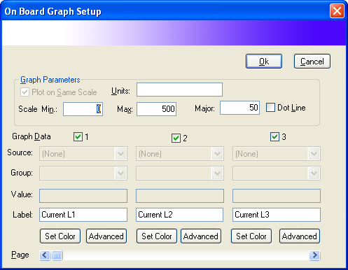
Figure 28 — On Board Graph Setup

2. Open

Opens a view window that was created earlier. A dialog appears listing all the windows available:

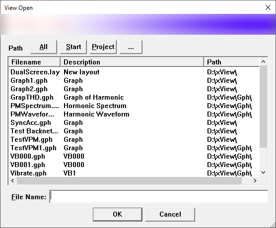
Figure 29 — Dialog for opening a window

The dialog lists the file name and the description given to each window when it was first created. Select the one you want and press to display it. Several entries can be selected at once and opened together. To move to a different directory, press to bring up the standard Open dialog.

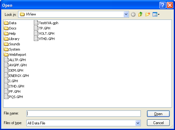
Figure 30 — Open dialog

3. Save

Saves the changes made to a window so that they take effect the next time it is displayed. If the window has not yet been named (Untitled), the system first shows a dialog asking for a name:

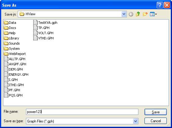
Figure 31 — Save As dialog

Enter the name of the window — which is also the name of the file it is saved to — in the File name box. Use something meaningful: a window graphing the power on all three phases might be called power123 or power, for example. The Save as type box sets the file extension automatically according to the window type.

Note

You do not need to type the extension: the system supplies the default one, as listed below.

Table 5 — File types

Window type	File extension
Instrument	*.IST
Graph	*.GPH
Harmonic Spectrum	*.SPT
Harmonic Waveform	*.WFM
Exported File	*.PRN
MMI File	*.DRW

4. Save As

Saves the window under a different name, leaving the original window unchanged. The dialog is the same as the one shown for Save.

Note

One use of Save As is to replicate a graph already built for one powermeter across several. With ten powermeters installed, for instance, build the graphs for the first one, then use Save As to produce the set for the second, one graph at a time, changing only the source of each line.

5. Print

Prints the window currently on screen (the active window). The following dialog appears:

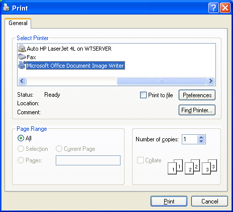
Figure 32 — Print dialog

Choose the printer under Select Printer, set the page range and number of copies, then press Print to start printing.

6. Advance Print

Prints several kinds of graph onto the same sheet of paper. Choose the layout you want and pick the graphs to print from the Name boxes.

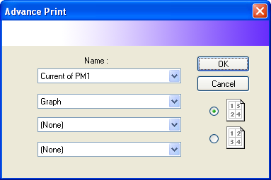
Figure 33 — Advance Print dialog

Select the windows to print from the Name dropdowns (up to four), set the print type in the dropdown below, and choose the page layout with the buttons on the right. Then press OK to print.

7. Print Preview

Previews the output before printing (available only for certain window types that display data).

8. Print Setup / Printer Setup

Sets the printer type and the print settings — for example whether to print portrait or landscape.

Tip: print graphs in landscape; the data is much easier to read that way.

Note

Printing under Windows requires the printer type to match the printer actually in use, or to be as close to it as possible. If you have trouble configuring the printer, see the Windows documentation under Settings > Devices > Printers & scanners.

9. Print Setup → Page Setup

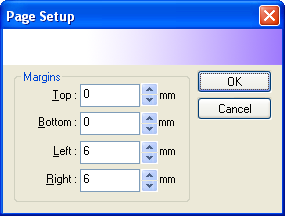
Figure 34 — Page Setup: paper margins

Sets the margins to leave when printing. All values are in millimetres. The defaults are Top/Bottom = 0 mm and Left/Right = 6 mm.

10. Communication Start

See the next section.

11. Communication Stop

Only a Supervisor may use this. It starts or temporarily stops data transfer with the devices in the system, such as SATEC Digital Powermeters, so that some other work can be done. For example, when the software is used as a portable analyser and you have returned from taking measurements at various sites, you would use Communication Stop while reviewing the data with no meter connected.

12. Communication Setup

Configures the communication channels and their settings, as shown.

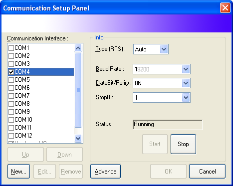
Figure 35 — Communication Setup panel

The panel contains:

1. Communication Interface — lists every COM port in the system. Tick the port you want to use, then set the values in the Info section on the right to match what is configured in the meter.

2. New — adds communication channels other than COM ports; see below.

3. Edit and Remove — change the details of, or delete, an additional channel.

4. Up and Down — order the additional channels. The standard channels cannot be reordered.

Settings for each channel (the Info section on the right)

1. Type (RTS) — the type of port used for the transfer. Some RS485 ports require this to be set.

2. Baud Rate — the communication speed, in bps (bits per second).

3. DataBit/Parity — the data length and the error checking used.

4. StopBit — the stop bit setting for the transfer.

5. Status — shows whether this channel is currently running (for example "Running").

6. Start and Stop — start or stop this channel, without affecting the others.

Other settings

1. Advance — additional communication settings that apply to every channel.

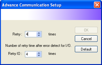
Figure 36 — Advance Communication Setup

Retry — how many times to repeat a read until it succeeds.

Retry IO — how many times to repeat a command sent to an output, such as switching a relay on or off.

Default — returns the settings to the program's standard values.

Notes

1. If you have entered something incorrectly and want the previous values back, Cancel out of the dialog and run the command again.

2. For adjusting the communication settings on each meter model, see that meter's manual. The standard settings are normally as shown above: 9600, 8N, 1.

3. For an RS-422 channel, nothing extra needs setting in the program, but the meter itself must be set to RS-422 communication (by DIP switch or by selection). See the meter's manual for details.